Taming Gradient Norm Spikes During LLM Scaling With Weave-Head Attention
TL;DR
- Problem: Large-scale LLM training suffers from gradient norm spikes that correlate with degraded learning dynamics and worse models.
- Method: Weave-Head adds content-aware, bidirectional head-to-head attention at the same token and jointly normalizes it with causal attention via an online softmax.
- Effect: At 4B and 7B, gradient norm spikes are sharply reduced; training loss descends faster; validation bits-per-byte improves. Gains grow with model size; effects are neutral at 1B.
- Cost: Extra FLOPs ≈ 0.1-0.5% in typical regimes; memory overhead ≈ 0.
Motivation
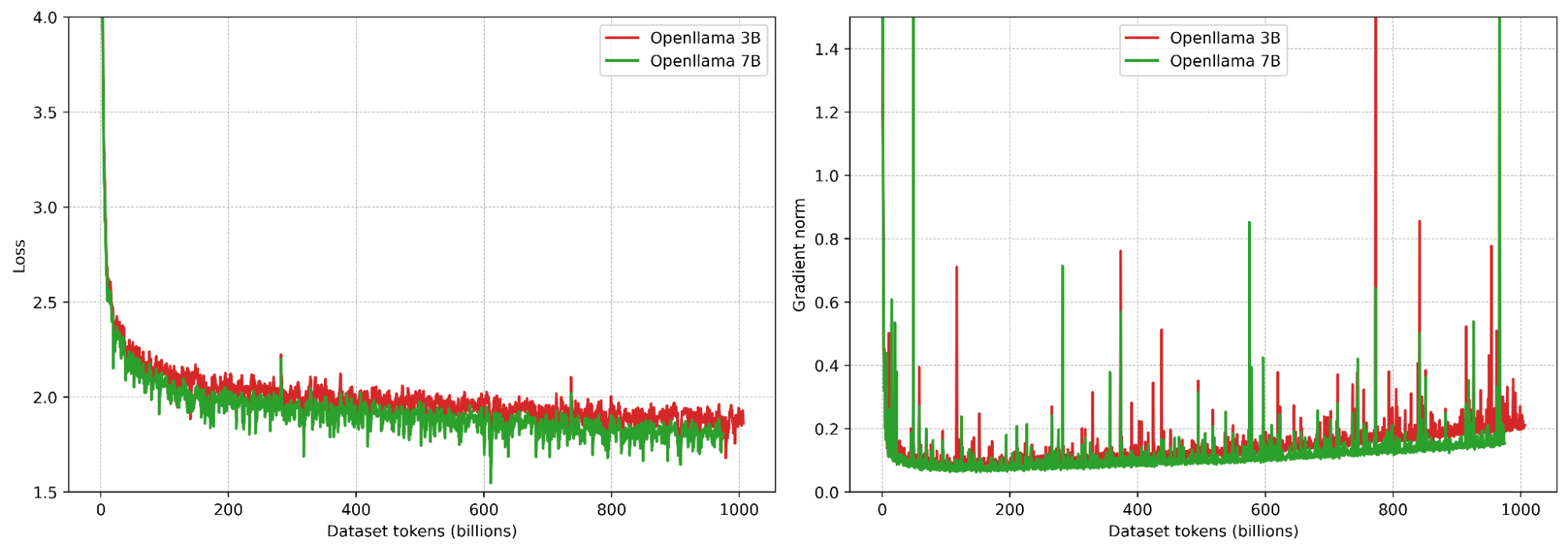
During large-scale LLM training, gradient norm spikes often appear and destabilize optimization—training jitters, convergence slows, and final quality suffers (see e.g. OPT[1], OpenLLaMA[2], PaLM[3], OLMo[4]). This issue becomes more severe as models scale up, making it a key challenge of scaling. Here's a concrete snapshot from training OpenLLaMA: both the 3B and 7B runs exhibit many gradient norm spikes.
Stabilization tricks exist, such as gradient norm clipping, qk normalization, warmup, data de-duplication, removing low-quality data, etc. But at large scale they may not fully eliminate spikes. This raised a question: perhaps information flow across heads is too weak. What if we let heads attend to each other?
Introducing Weave-Head Attention
Weave-Head augments standard Multi-Head Attention (MHA) with bidirectional cross-head attention within each token. Intuitively, before a head commits to a causal distribution over the past, it first consults other heads at the same token to aggregate their evidence. Concretely, Weave-Head performs:
- Head-to-head attention (at the same token/position) (heads at the same position attend to each other)
- Causal attention (each head attends over previous positions).
- Online softmax that jointly normalizes “other heads @ same token” and “same head over time.” with zero memory overhead.
Why this helps (intuition)
- Shorter feedback path. In vanilla MHA, cross-head coordination happens only after attention via the output projection. Weave-Head moves that coordination earlier—into the attention computation itself—so signals about which heads are reliable get back-propagated to \(Q/K\) faster, improving information flow.
- Content-aware mixing. Unlike fixed, content-agnostic head mixing (cf. Talking-Heads [5]), Weave-Head's cross-head links are content-dependent (\(q\!\cdot\!k\) across heads), with almost zero overhead.
- Keep specialization without collapse. Heads can be grouped (syntax/semantics/long-range) and masked to allow strong cross-group communication while preserving within-group expertise.
Near-Zero Overhead
Summary. Extra FLOPs ≈ \(\frac{H}{6D + S}\); memory ≈ 0 (continue the online softmax to fuse cross-head terms). Here \(H\)=heads, \(D\)=model dim, \(S\)=sequence length. In typical regimes this is ≈ 0.1-0.5% FLOPs.
Example
\(D{=}4096,\,H{=}32,\,S{=}2048\): Weave adds \(\frac{H}{6D + S} = \frac{32}{6 \times 4096 + 2048} \approx 0.12\%\) extra FLOPs. Memory-wise, Weave-Head uses zero extra memory: compute causal attention and continue the online softmax with the cross-head terms.
Show derivation
Let \(B\) = batch, \(S\) = sequence length, \(D\) = model dim, \(H\) = num of heads, \(K\) = head dim. Count a multiply-add as 2 FLOPs.
Baseline (per layer, forward)
- Projections \(Q,K,V\): \(3\) GEMMs \(\Rightarrow 6BSD^2\)
- Scores \(QK^\top\): \(2BHS^2K = 2BS^2D\)
- Apply weights to \(V\): \(2BS^2D\)
- Output projection \(O\): \(2BSD^2\)
Attention total: \(8BSD^2 + 4BS^2D\). MLP (expansion 4): \(16BSD^2\).
Baseline FLOPs: \(\;24\,B S D^2 + 4\,B S^2 D\).
Weave-Head (additional, per layer, forward)
At each token, cross-head attention computes:
- Cross-head scores: \(2\,B S H^2 K = 2\,B S H D\)
- Weights-values product: \(2\,B S H^2 K = 2\,B S H D\)
Weave overhead: \(\approx 4\,B S H D\).
Overhead ratio (vs. baseline): \(\displaystyle \frac{4\,B S H D}{24\,B S D^2 + 4\,B S^2 D} = \frac{H}{6D + S}\).
Experiments
Setting. We train LLMs at 1.5x Chinchilla optimal [6] (≈30 tokens per parameter). We compare Baseline and Weave-Head across model sizes. The plots report training loss, gradient norm (average + per layer), and validation bits per byte (bpb).
The model architecture follows a LLaMA-2 style design (dense; one MLP and one self-attention per layer). We trained three model sizes: 1B, 4B, and 7B.
Experimental setup (click to expand)
| Global batch size | 512 sequences x 2048 tokens (per step) |
|---|---|
| Sequence length | 2048 |
| Learning rate | 2e-4, linear warmup for 200 steps and cosine decay to 10% |
| Hardware | Google Cloud TPUv4-512 |
| Sharding | FSDP + SP (ring) |
| Normalization | Pre RMS norm, QK RMS norm |
| Training data | Mixture of fineweb, starcoder, wikipedia, arxiv and books. Maximum one epoch, no repeating |
| Validation data | Hold-out split of the training data |
| Tokenizer | LLaMA 3 tokenizer |
Model configurations (click to expand)
| Model | Layers | Heads | Head dim |
|---|---|---|---|
| 1B | 20 | 16 | 128 |
| 4B | 30 | 28 | 128 |
| 7B | 34 | 32 | 128 |
We now show results at 4B and 7B side-by-side from four angles: gradient norm, per-layer gradient norm, training loss, and validation bits per byte (bpb).
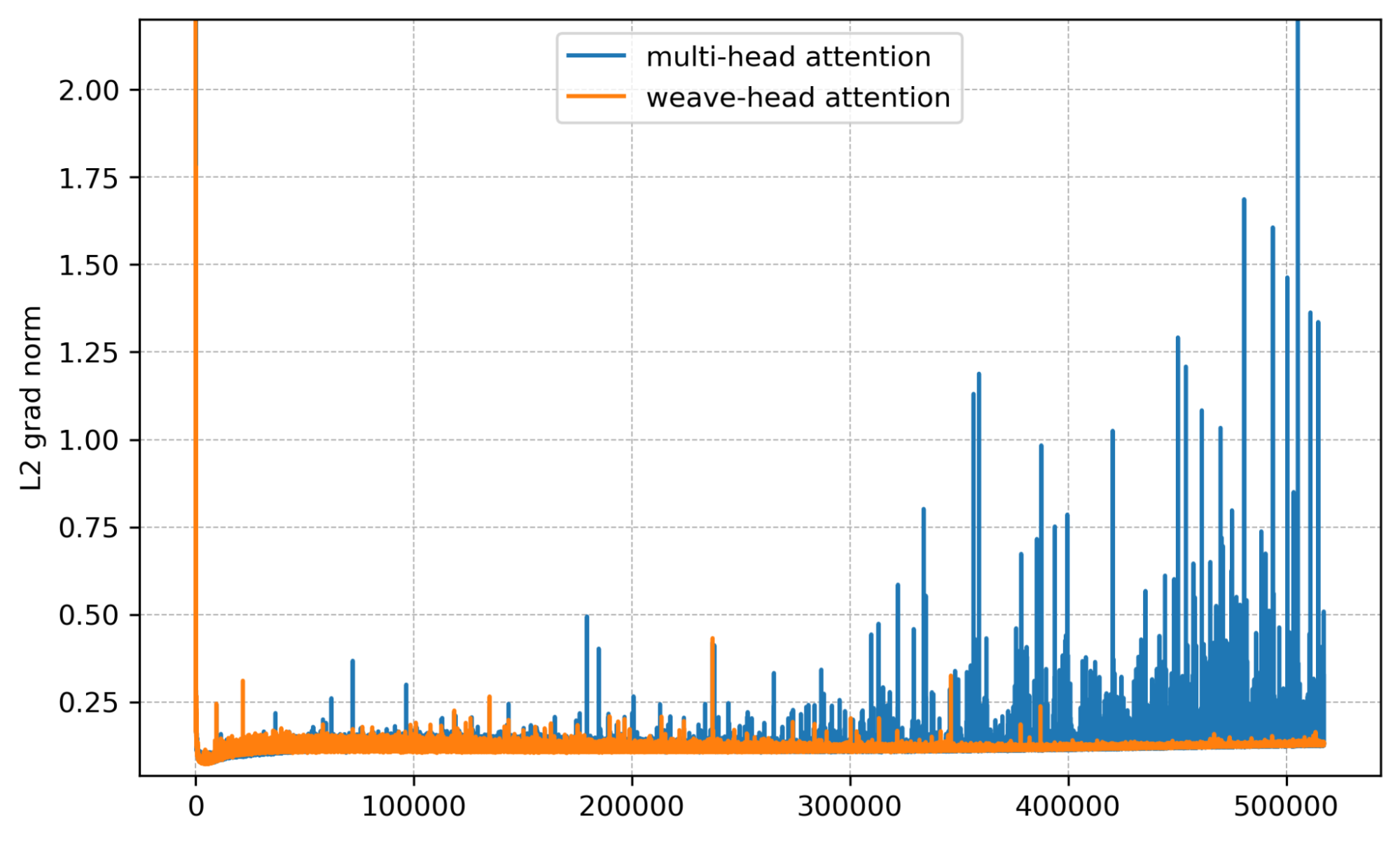
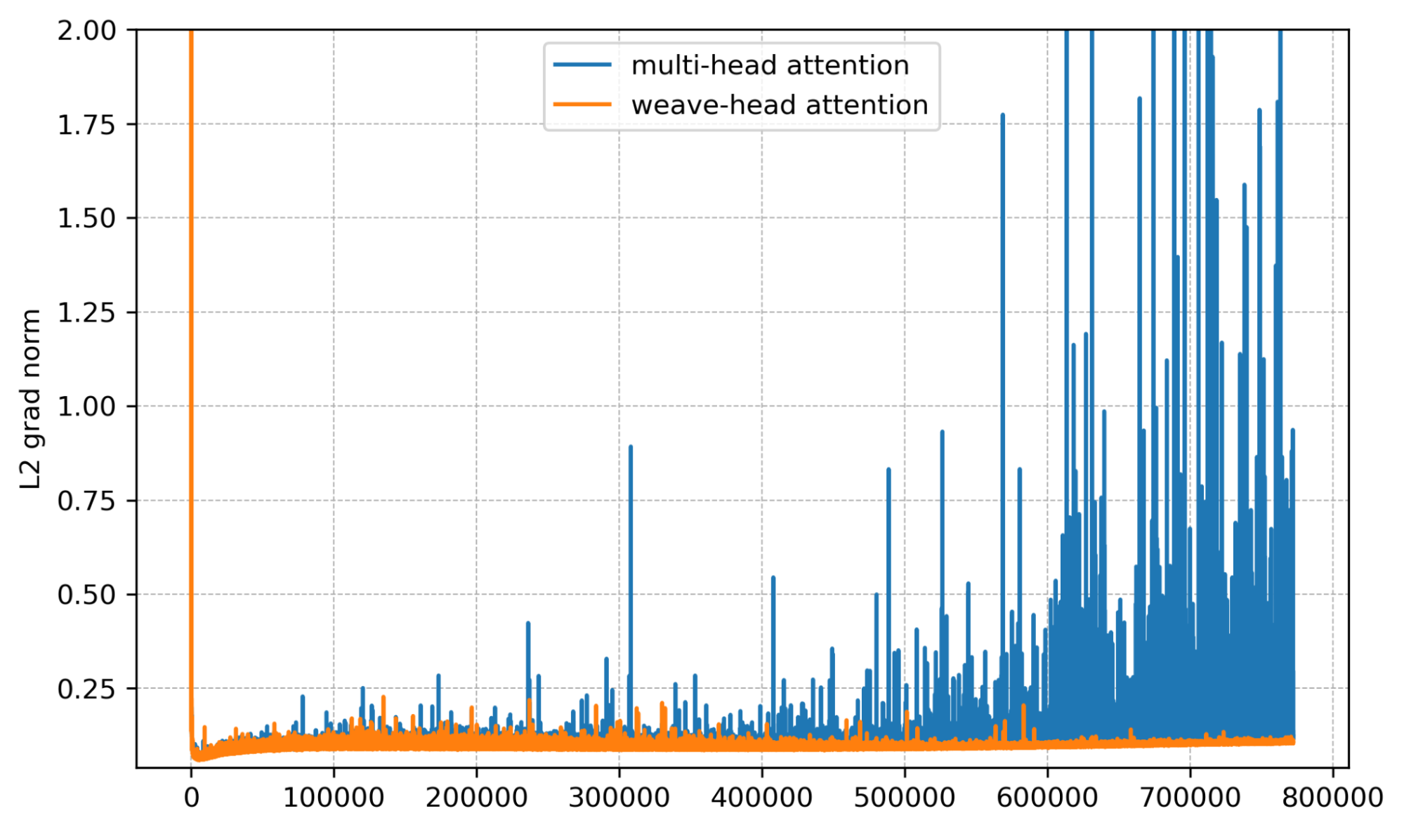
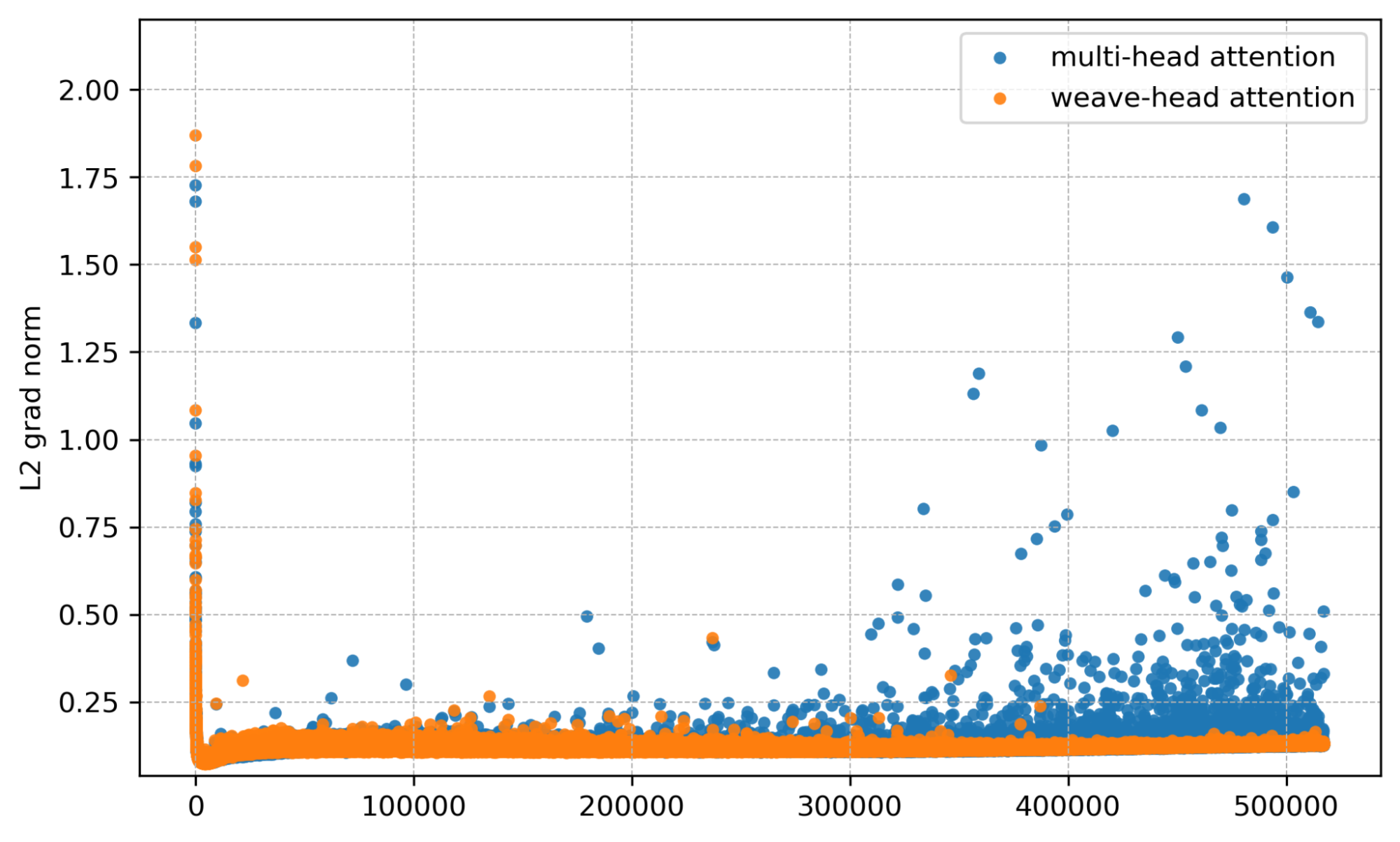
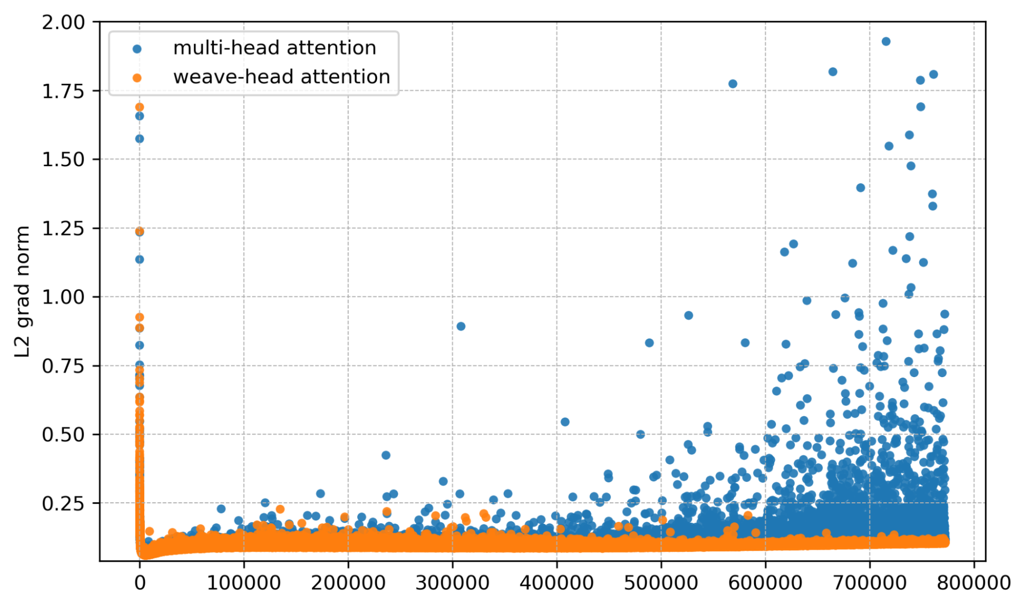
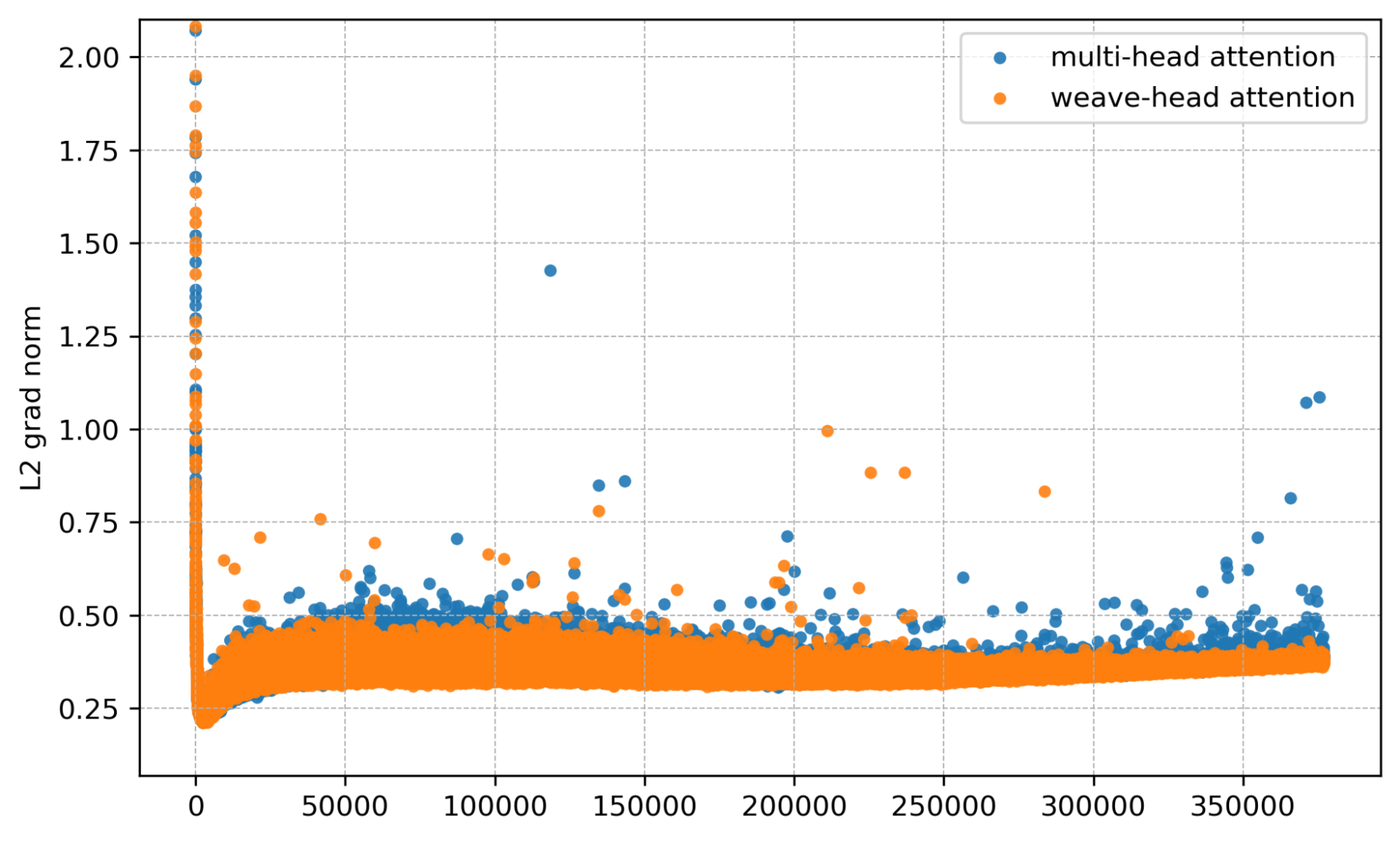
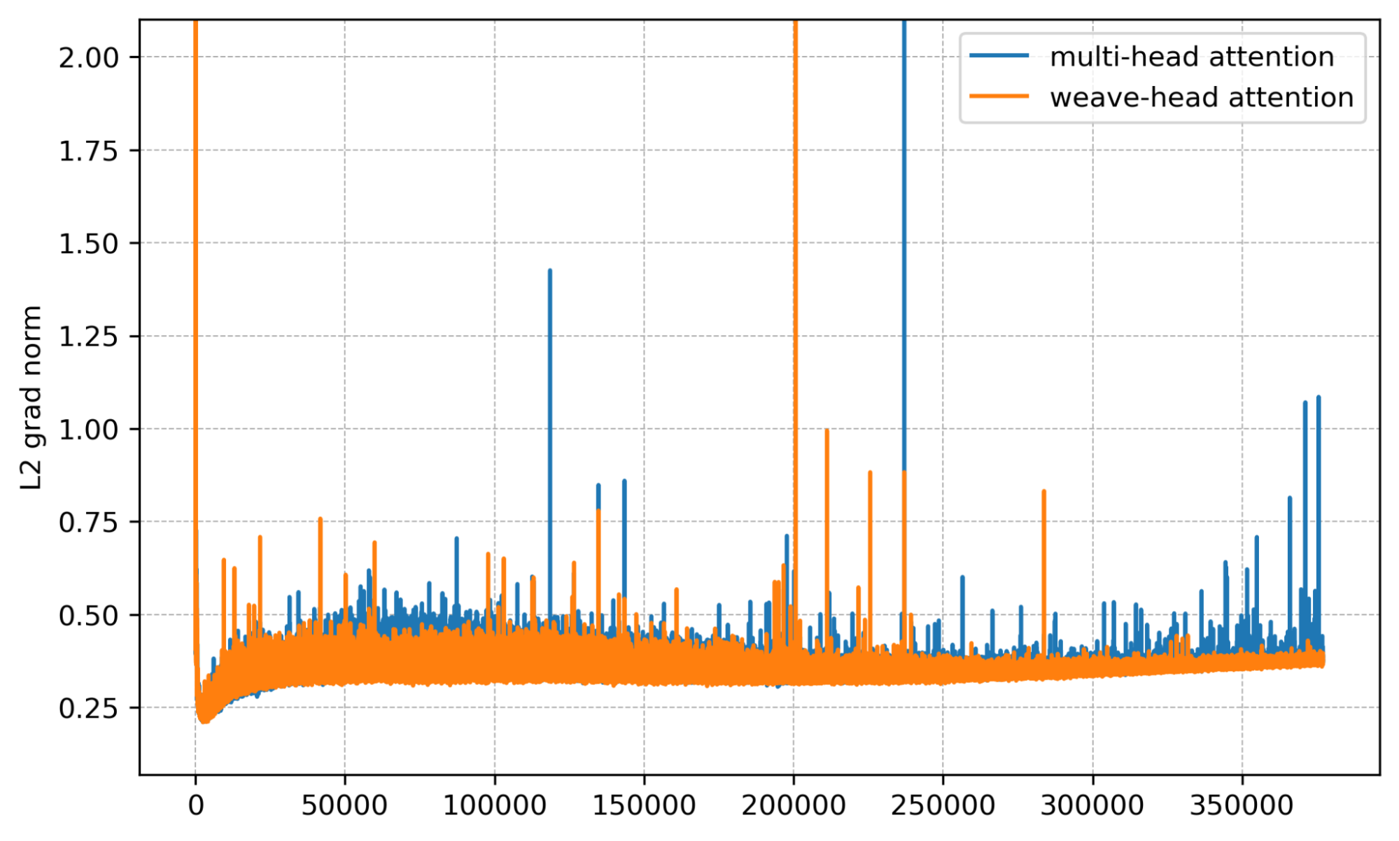
Mean gradient norm. Spikes are sharply reduced with Weave-Head.
Per-layer view. Baseline shows bursty multi-layer spikes; Weave-Head shows none.
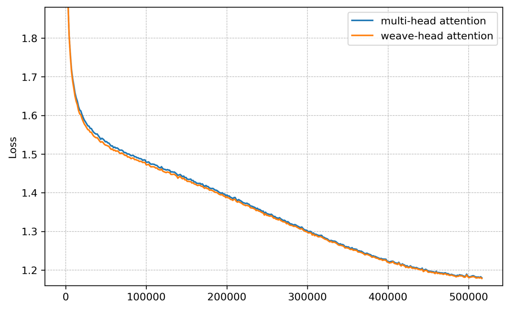
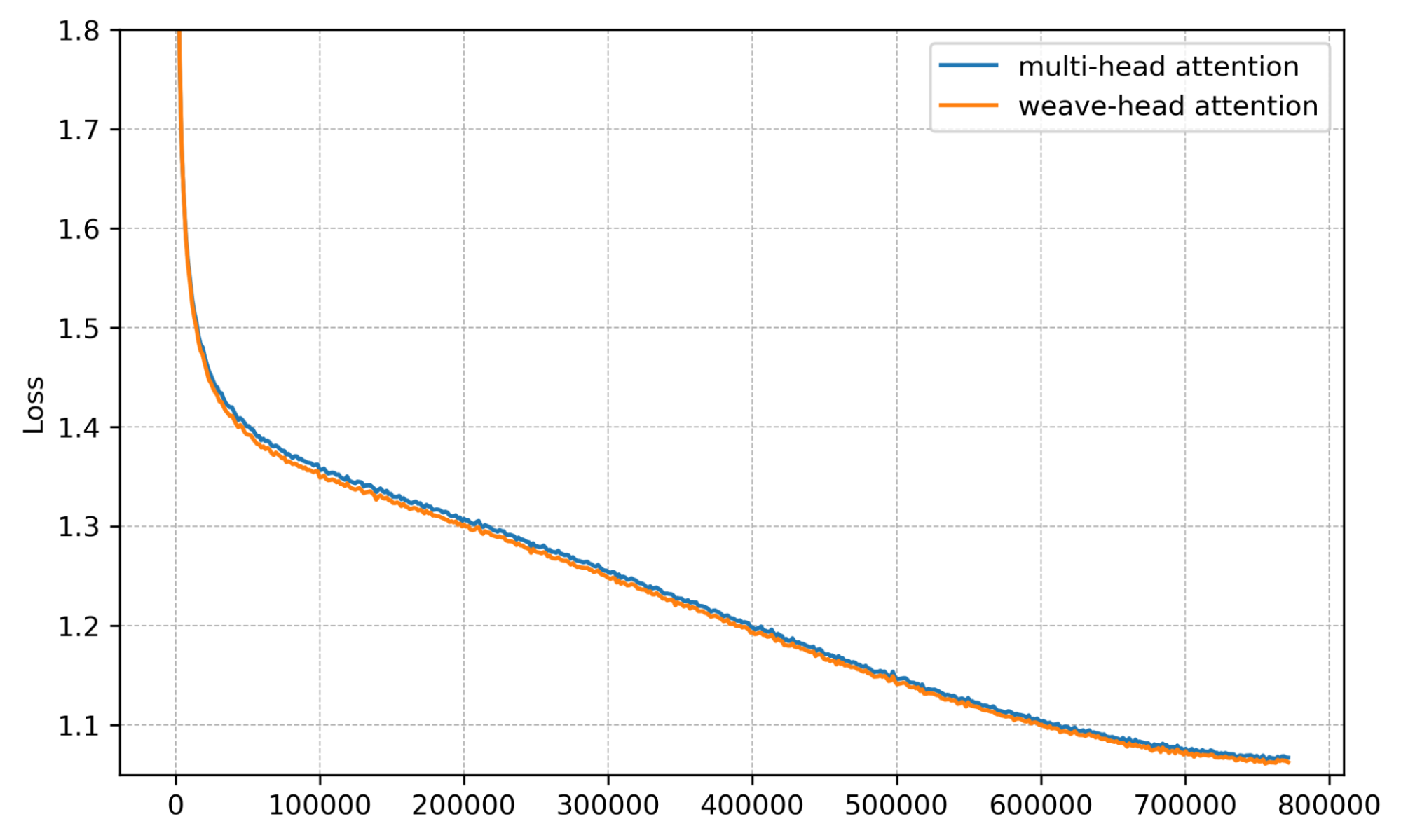
Training loss. Loss decreases faster and to a lower value with Weave-Head.
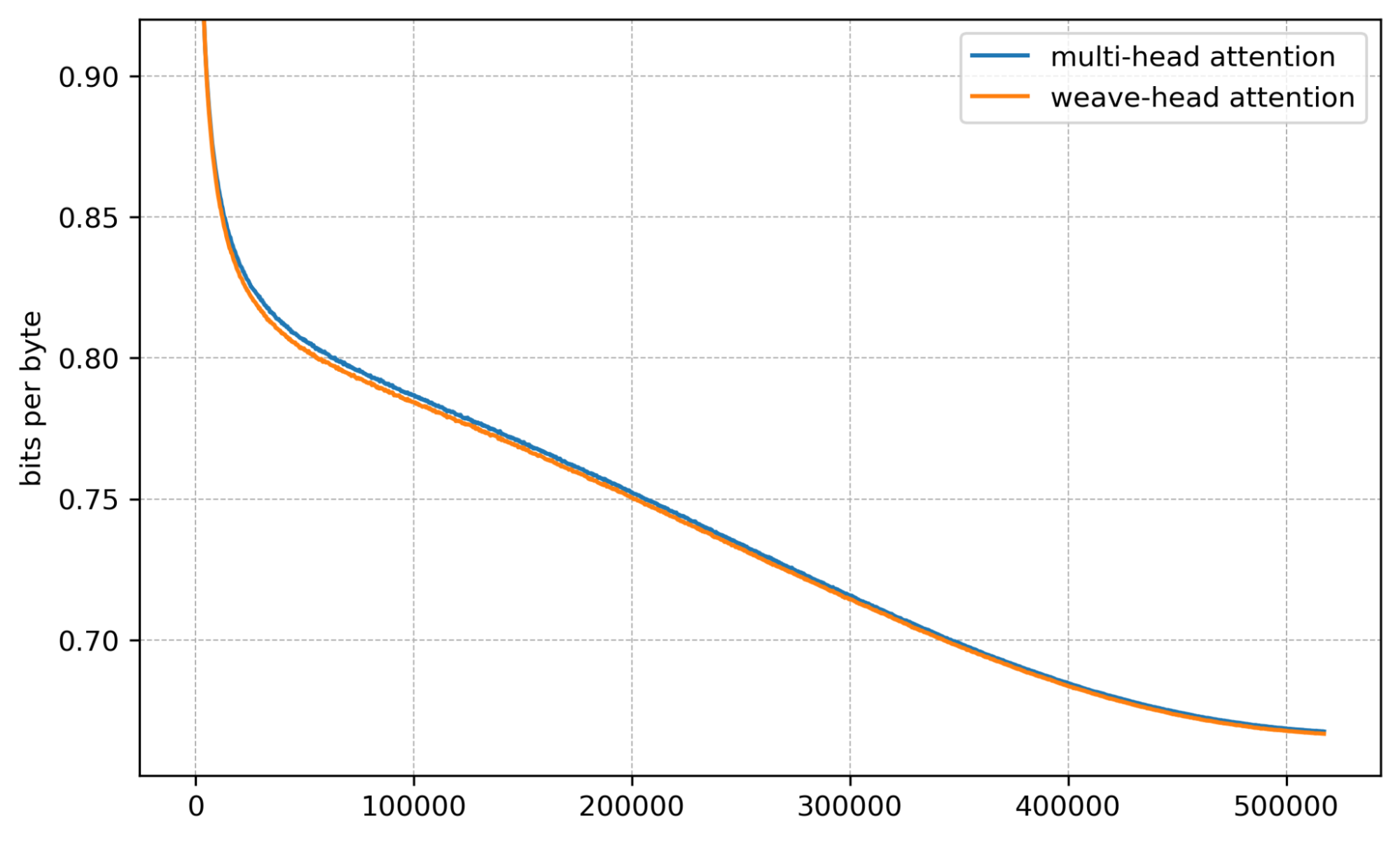
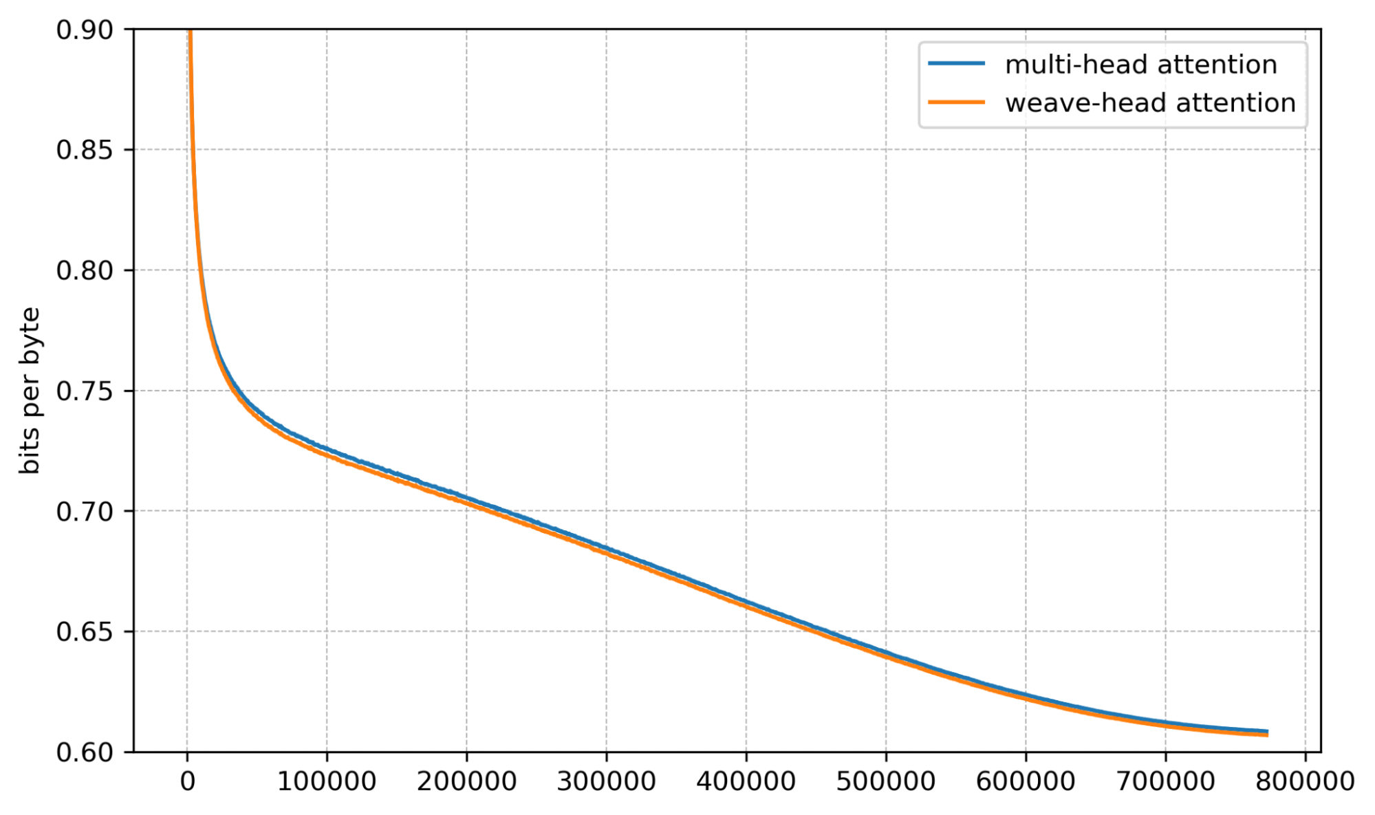
Bits per byte. Validation bpb is consistently lower with Weave-Head.
Small scale (1B): minimal effect (click to expand)
Discussion
- Scale matters. The benefits grow with model size, which is where gradient norm issues are most troublesome. Scaling laws is a potential area where Weave-Head could provide further benefits.
- Future work. Can we amplify gains at small scale via better head grouping/masking? How does Weave-Head interact with long-context variants? How will it perform at larger scales? How will it perform with different input modalities (e.g., images, video)?
Jax Code
This code implements Weave-Head Attention in Jax. In this case, XLA provides adequate fusion of head-to-head and causal attention. Nevertheless, to approach hardware-limited performance, a kernel in Pallas/CUDA is recommended.
def weave_head_attention(q_BHTK: jax.Array, k_BHTK: jax.Array, v_BHTK: jax.Array) -> jax.Array:
    B, H, T, K = q_BHTK.shape
    assert k_BHTK.shape == (B, H, T, K) and v_BHTK.shape == (B, H, T, K)

    # same-token cross-head (xh)
    q_bHK = q_BHTK.transpose(0, 2, 1, 3).reshape(B * T, H, K)
    k_bHK = k_BHTK.transpose(0, 2, 1, 3).reshape(B * T, H, K)
    v_bHK = v_BHTK.transpose(0, 2, 1, 3).reshape(B * T, H, K)

    scale = 1.0 / jnp.sqrt(K)
    logits_xh = jnp.einsum("bHK,bQK->bHQ", q_bHK, k_bHK) * scale
    m_xh = jnp.max(logits_xh, axis=-1, keepdims=True)
    w_xh = jnp.exp(logits_xh - m_xh)
    den_xh = jnp.maximum(jnp.sum(w_xh, axis=-1), 1e-9)
    num_xh_bHK = jnp.einsum("bHQ,bQK->bHK", w_xh, v_bHK)

    m_xh = m_xh.reshape(B, T, H, 1)
    den_xh = den_xh.reshape(B, T, H)
    num_xh = num_xh_bHK.reshape(B, T, H, K)

    # causal across tokens (per head)
    tri_TS = jnp.tril(jnp.ones((T, T), dtype=bool))
    logits_causal = jnp.einsum("BHTK,BHSK->BHTS", q_BHTK, k_BHTK) * scale
    logits_causal = jnp.where(tri_TS[None, None, :, :], logits_causal, -jnp.inf)

    m_causal = jnp.max(logits_causal, axis=-1, keepdims=True)
    w_causal = jnp.exp(logits_causal - m_causal)
    den_causal = jnp.maximum(jnp.sum(w_causal, axis=-1), 1e-9)
    num_causal = jnp.einsum("BHTS,BHSK->BHTK", w_causal, v_BHTK)

    m_causal = m_causal.transpose(0, 2, 1, 3)
    den_causal = den_causal.transpose(0, 2, 1)
    num_causal = num_causal.transpose(0, 2, 1, 3)

    # fuse via online softmax
    m_final = jnp.maximum(m_xh, m_causal)
    num_final = num_xh * jnp.exp(m_xh - m_final) + num_causal * jnp.exp(m_causal - m_final)
    den_final = (
        den_xh * jnp.exp(m_xh.squeeze(-1) - m_final.squeeze(-1)) +
        den_causal * jnp.exp(m_causal.squeeze(-1) - m_final.squeeze(-1))
    )
    den_final = jnp.maximum(den_final, 1e-9)

    return (num_final / den_final[..., None]).transpose(0, 2, 1, 3)
Acknowledgments
Many thanks to TPU Research Cloud (TRC) and Google Cloud research credits for supporting the experiments behind this simple idea I first prototyped in graduate school. Over Labor Day weekend, I finally had some personal time to write this blog.
References
- OPT — Zhang et al., “OPT: Open Pre-trained Transformer Language Models,” (2022). arXiv:2205.01068
- OpenLLaMA — OpenLM Research, “OpenLLaMA: An Open Reproduction of LLaMA” (2023). Project
- PaLM — Chowdhery et al., “PaLM: Scaling Language Modeling with Pathways” (2022). arXiv:2204.02311
- OLMo 2 — AI2, “OLMo 2 Technical Report” (2025). Project
- Talking-Heads Attention — Shazeer et al., “Talking-Heads Attention” (2020). arXiv:2003.02436
- Chinchilla — Hoffmann et al., “Training Compute-Optimal Large Language Models” (2022). arXiv:2203.15556
Citing this blog post
If this blog is useful and you'd like to cite it:
@misc{liu2025weave,
      title        = {Taming Gradient Norm Spikes During LLM Scaling With Weave-Head Attention},
      author       = {Hao Liu},
      year         = {2025},
      howpublished = {\url{https://haoliu.ai/blog/weave-head.html}}
    }
Back to top
Blog
Home